Epi Vignettes: Longitudinal or Multilevel Study
A brief synopsis of epidemiologic study design and methods with sample analytic code in R.
In this third installment in the series, I discuss study designs with correlated observations and appropriate analytic techniques. As before, the intention of this series is to:
- Briefly describe the study design.
- Qualitatively talk about the analysis strategy.
- Quantitatively demonstrate the analysis and provide sample R code.
- Study design: Longitudinal or Multilevel. In this study design, the observations in the data may be correlated with each other. While this occurs via different mechanisms depending on the type of study, the analysis is similar; therefore these concepts are often presented together. Nevertheless, it is important to recognize how correlation occurs for each type of study before proceeding to analytic strategy. In a longitudinal or repeated outcomes measures study, an individual contributes multiple observations to the data as they have an outcome that is measured on two or more occasions. Hence any exposure/outcome relationship within that individual needs to be accounted for separately from the exposure/outcome relationship between individuals, as each individual may respond to an exposure differently. In a multilevel (aka hierarchical) study, a contextual unit contributes multiple observations to the data, as two or more individuals are located within these units. More concretely, if a study examined neighborhood effects, neighborhoods are composed of individuals, hence any exposure/outcome relationship within the individuals needs to be accounted for separately within each correlated unit (i.e., the neighborhood). In all cases, statistical techniques are needed to account for this correlation.
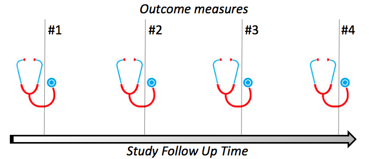
- Data Description: Assume a binary exposure, two types of outcomes (continuous for the longitudinal study and binary for the multilevel study), and several covariates that are potential confounders. Chiefly applicable to a longitudinal study, the data should be organized in a "long" format whereby each individual outcome is a unique observation. For example, for a repeated measures study with five total outcome measures, this would translate to five separate observations for each individual, with a single outcome variable and a time variable coded as one through five. Of course presence of missing data means fewer observations per individual.
- Goal of Analysis: Describe the relationship between the exposure and outcome accounting for correlation of observations. This relationship can be described in terms of global effects (its effect is equivalent across everyone in the study) and is termed a fixed or marginal effect, or can be described in terms of a varying effect (its effect differs by the individual in the repeated measures study or the contextual unit in the multilevel study, termed group hereafter) and is termed a random effect. Fixed effects are akin to the standard coefficient estimates in single-level, typical regression analysis, and therefore are more intuitive to interpret. Random effects are frequently used describe sources of variation in the data, and therefore do not normally have coefficient estimates presented, but rather estimates based on the group variance.
- Statistical Techniques: Assuming we would like to describe both fixed and random effects, we will fit a mixed effect model. If the interest is to describe fixed effects alone, the reader may wish to use generalized estimating equations to fit the model, however as I am interested in mixed effects, therefore will deal only with likelihood based estimation to fit the model (see this blog post I previously wrote for a more detailed discussion). Model building is treated as an iterative process that starts out with the simplest model first and then adds covariates. Model convergence may be challenging in mixed effects regression. Continuous covariates may need to be mean centered or scaled (such as through a log transformation), additionally there may be collinearity introduced by multiple group predictors, therefore simpler models may be preferred. In short, these are not trivial models. Click here for a useful comparison of modeling approaches among the major statistical platforms.
- Mixed effects regression with a continuous outcome (linear mixed effects regression): This technique is appropriate when the outcome is continuous and can be represented by a linear relationship, as in the example given above for a longitudinal study). The first step is to check for correlation among the observations in the dataset and if significant correlation is detected the model building process can proceed. In order to check for correlation among observations, an empty model is fit that describes only the outcome and the group unit (fit as a random intercept, or allowed to differ for each group). Assuming significant correlation is detected, an appropriate covariance structure should be chosen (e.g., unstructured, symmetric, autoregressive, etc.) using REML estimation. Next, the exposure can be introduced to check for a crude relationship with the outcome. At this point, the researcher needs to decide whether the exposure is a fixed effect (one with a population level effect), a random effect (one with a group specific effect), or both (fixed and random effects). Potential confounders can also be introduced at this point with final estimates made using ML estimation. Typically in longitudinal analyses, we are interested in interacting the exposure with time to assess whether there are differences over time between groups. To do this, two nested models are built: one with an interaction term and one without. If the result of the Type 3 test for interaction is significant, then the interaction term is appropriate and one can conclude there likely are differences over time between groups by the exposure.
- Mixed effects regression with a binary outcome (generalized linear mixed effects regression): This technique is appropriate when the outcome is binary and can be represented by a generalized linear relationship (through a logit link function), as in the example given above for a multilevel study. As before, the first step is to check for correlation among the observations in the dataset and if significant correlation is detected the model building process can proceed. In order to check for correlation among observations, an empty model is fit that describes only the outcome and the group unit (fit as a random intercept, or allowed to differ for each group). Assuming significant correlation is detected, an appropriate covariance structure should be chosen (e.g., unstructured, symmetric, autoregressive, etc.) using REML estimation. Note: the R procedures shown below assume unstructured correlation, which unfortunately cannot be changed in the package LME4 at present. Likewise, REML estimation for model comparison is also not possible currently. Next, the exposure can be introduced to check for a crude relationship with the outcome. At this point, the researcher needs to decide whether the exposure is a fixed effect (one with a population level effect), a random effect (one with a group specific effect), or both (fixed and random effects). Potential confounders can also be introduced at this point with final estimates made using ML estimation. In the multilevel example from before, examining the change in group level variance can be done to assess the relationship of the predictors on the outcome, where reduction in area level variance probably indicates more meaningful predictors
Sample codes in R
Mean center a continuous variable
variable_centered = scale(variable, center=T, scale=F)
Linear mixed effects regression (package:nlme)
Empty model with random subject intercept
model = lme(outcome ~ 1, random=~1| group, data= dataset, method="ML")
Choosing a covariance structure: select model with lowest AIC/BIC
model = lme(outcome ~ 1, random=~1| group , data= dataset, method="REML") #unstructured
model = lme(outcome ~ 1, random=~1| group, correlation=corSymm(), data= dataset, method="REML") #symmetric
model = lme(outcome ~ 1, random=~1| group, correlation=corAR1(), data= dataset, method="REML") #autoregressive
model = lme(outcome ~ 1, random=~1| group, correlation=corCompSymm(), data= dataset, method="REML") #compound symmetry
Exposure*time interaction
modelInteraction = lme(outcome ~ time*exposure + covariates, random=~1|group, correlation=structure, data= dataset, method="ML")
modelNoInteraction = lme(Weight ~ time + exposure + covariates, random=~1| group, correlation= structure, data= dataset, method="ML")
anova(modelInteraction,modelNoInteraction)
Linear mixed effects regression (package:lm4)
Empty model with random subject intercept
model = lmer(outcome ~ (1 | group), data= dataset, REML=F)
Full model with random subject intercept
model = lmer(outcome ~ (1 | group) + Time*exposure + covariates, data= dataset, REML=F)
Generalized linear mixed effects regression (package:lme4)
Empty model with random group intercept
model = glmer(outcome ~ (1 | group), family=binomial(), data=dataset)
Crude model with random group intercept and fixed effect
model = glmer(outcome ~ (1 | group) + exposure, family=binomial(), data=dataset)
Crude model with random group intercept and random effect
model = glmer(outcome ~ (1 + exposure | group), family=binomial(), data=dataset)
Crude model with random group intercept and fixed + random effect
model = glmer(outcome ~ (1 + exposure | group) + exposure, family=binomial(), data=dataset)
Fully adjusted model with random group intercept and fixed + random effect
model = glmer(outcome ~ (1 + exposure | group) + exposure + covariates, family=binomial(), data=dataset)
Odds ratios and CI estimates for fixed effects
exp(fixef(model))
exp(confint.merMod(model, method="Wald"))
Cite: Goldstein ND. Epi Vignettes: Longitudinal or Multilevel Study. Aug 12, 2015. DOI: 10.17918/goldsteinepi.