Sensitivity analysis for residual confounding
Suppose you are conducting an epidemiological analysis of the relationship between an exposure and a biologic outcome (disease). You find there is effect modification, say by race, in the exposure/outcome relationship. If there is no biological basis for a racial difference, which is often the case, how can this be? There are many theoretical possibilities: differential misclassification, random chance, and so on. Let's assume the study was a well designed and conducted observational study that maximized internal validity. Sure, random chance could factor, or more likely, there may be unmeasured confounding.
Residual confounding (the result of a latent confounder or confounders) can often cause divergent results and apparent effect modification. It does not need to be particular to a single study: perhaps you are comparing your study to published literature and one study controlled for an important variable another did not. Or there was a key difference in how an exposure was assessed that introduced confounding. If there is no biologic basis for results differing, residual confounding should be suspected before a true difference is concluded.
For users of causal diagrams (including DAGs) latent confounders are often depicted as the big "U," or as a friend of mine would say, a big cop-out. Didactically, U represents a universe of known (but mismeasured) and unknown confounders. In the search for possible attributes of residual confounding it is often useful to have a quantitative description of the latent confounder(s) U: what is the strength of U, and how does its prevalence differ between exposure groups? Knowing the strength of U indicates the magnitude of its effect, and the prevalence allows a directed search for potential factors.
To quantify U, we can conduct a sensitivity analysis of residual confounding using the proposed methods in the obsSens package in R. There are several assumptions to specify:
- A regression model that specifies the exposure and outcome relationship of interest controlling for known confounding.
- What variable types are the exposure, outcome, and latent confounder? These can either be continuous or categorical (or even a survival object for the outcome). We'll assume all are categorical (dichotomous) for simplicity.
- What is the hypothesized true relationship between the exposure and outcome? If the estimates are diverging by effect modification between groups, is one group more believable than the other? Perhaps the true relationship is somewhere in between? Or is there external evidence of the true relationship? This hypothesized true relationship serves as the target in the sensitivity analysis.
- What is the plausible range of the strength of U on the outcome?
- What are the plausible ranges for the prevalence proportions of U in each exposure group?
Of course the object of the sensitivity analysis is to get at the answers to #4 and #5 from above, right? But in order to deduce information about U some starting assumptions are needed. However, these are quite broad. You may assume U is somewhere between 2 and 40, and the prevalence is between 0 and 100%. The output from the obsSens procedures will be a table with adjusted relationship between the exposure and outcome, and then the user needs to establish which measures of the strength of U and prevalence proportions in the exposure groups makes the most sense.
Here's an example call to the sensitivity analysis:
obsSensCCC(model, which=2, g0=seq(2,10,4), p0=seq(0,1,0.2), p1=seq(0,1,0.2), logOdds=F)
where:
- obsSensCCC = a sensitivity analysis for three categorical variables (outcome Y, exposure X, and latent confounder U)
- model = the regression model
- which = the parameter in the regression model that specifies the exposure
- g0 = strength of the relationship between U and the outcome (specified here as an odds ratio); also called gamma
- p0 = prevalence of U in unexposed group (or when exposure = 0)
- p1 = prevalence of U in the exposed group (or when exposure = 1)
- logOdds = whether log of the odds or the odds ratio should be returned
And example output:
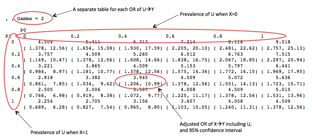
This is pretty useful, but there is potentially a lot of information to wade through. Additionally, there will be multiple points on each table where the hypothesized true relationship between the exposure and outcome adjusted for U are found, depending on the strength of U and prevalence of U in the exposure. Therefore, it may help to create a simplified table that allows for a more directed search for plausible values of U.
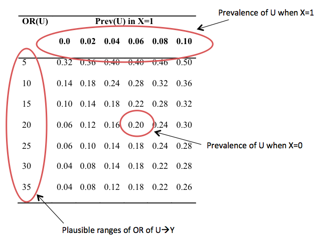
To construct this table, the columns correspond to the prevalence of U when the exposure is present; and the value of the rows is the prevalence of U when the exposure is not present, where each row is particular to the strength of U on the outcome. To choose the appropriate value, we search the sensitivity analysis tables for when the adjusted OR of X on Y is close to the hypothesized value. After this table is constructed, one searches for where the prevalence estimates begin to stabilize to find the most plausible values. The relationship of the unadjusted (for U) X with Y to the adjusted (for U) X with Y indicates the direction of confounding, and the strength of U and prevalence of U in X is determined from this sensitivity analysis.
A drawback to this approach is it assumes a net effect from U. In fact, U may be the result of many latent confounders which have very different effects. One useful rule of thumb: if there is strong confounding present in the dataset, U also like has strong effects; and if there is weak confounding present, U is likely weak.
Cite: Goldstein ND. Sensitivity analysis for residual confounding. Oct 5, 2015. DOI: 10.17918/goldsteinepi.