Social Network Analysis in Epidemiology: Part 3
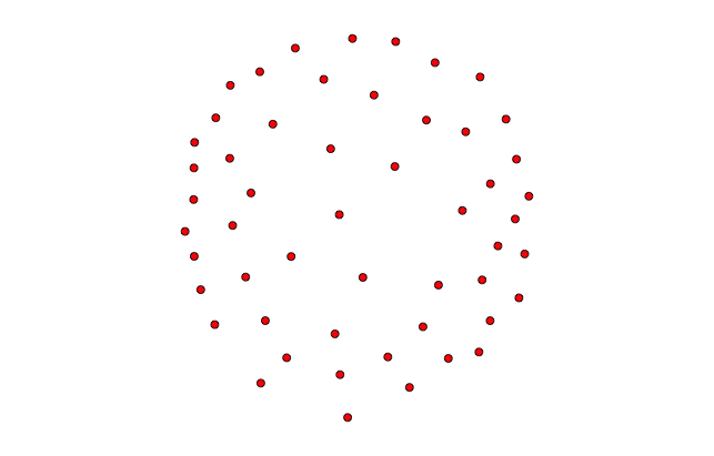
Using social networks to model infectious disease transmission requires not only the parameters of what causes disease to spread (and not spread) but also a representative network of individuals. To create this representative network requires data. We will assume true network census data are not available and data are thus egocentric. Therefore the first step is to construct a network that represents accurate "connectivity": the relationships between people in the network model should not be due to chance alone but represent some actual process of forming and dissolving relationships, known as assortative mixing. These patterns of interactions may be related to sexual characteristics, environmental characteristics, parental characteristics, caregiver characteristics, and so on. We can use the statnet package in R to do the modeling, which is included in EpiModel. The authors of statnet have also written a tutorial on modeling exponential-family random graph models in R; specifically section 7 for working with egocentric data.
In essence, we want to model the probability of relationships occurring between nodes, which may be a function of nodal attributes (gender, race, etc.) as well as the propensity for certain network configurations (triangle formation). In specifying the model in statnet, we can look at different selection processes of relationships forming:
- Edges: the number of relationships in the network
- Attributes: characteristics of the nodes governing relationships between nodal attributes (nodefactor) and within nodal attributes (nodematch, aka homophily)
- As an important aside, when assigning more than one attribute, the values are inter-dependent. For example, suppose you wish to create a network of 100 males and females evenly split in 2 locations. You would first assign the two locations, and then within each of the locations, assign 25 males and 25 females.
- Concurrent: multiple partners for a given node (but not necessarily transitivity)
- GWESP: multiple partners for a given node (shared partners, transitivity)
- Many other network terms are available; see help("ergm-terms")
We can extend these models by also considering relationship formation and dissolution. This extends the network from being cross-sectional (where we only have data on a snapshot in time, the presence of a relationship) to dynamic (where we have additional information about relationships forming and dissolving). The prevalence of relationships at any given time will be a function of the incidence of relationships forming multiplied by the duration that relationships last (the inverse of dissolution). This is the well-known formula: prevalence = incidence X duration. Another extension to these models is adding new people into the network (some "birth" rate) and removing people form the network (some "death" rate). To build these models requires egocentric data on what the relationship patterns may be, as well as whether the model should be static (ERGM) or dynamic (STERGM).
In the simplest dynamic network, we need data ascribing:
- The network size and whether it is directed or undirected.
- Specified as network.initialize(
, directed = .) - The average number of edges (e.g., relationships) per node in the network at any given point in time. This can be calculated based on the mean degree or from the degree distribution, if available. Since an edge connects two nodes, this number is divided by 2.
- Edges = mean_degree*num_nodes / 2
- Edges = sum(degree_distribution*degrees) / 2/li>
- Specified as the target.stats to the edges term in the formation model.
- The average duration of an edge (e.g., relationship).
- Specified as the coef.diss in terms of number of times steps in the model (units of time steps are arbitrary).
The network is first built using the function netest (or for static networks the function ergm). And then is simulated over some number of time steps using the function netdx (or simulate for static networks), where the edges are actually estimated in the model. This edges-only model is a random process, and does not include any restrictions based on concurrency (multiple partners for a given node). The degree distribution in this edges-only model will follow a Poisson distribution with the rate parameter set to the mean degree. To get a sense for what this degree distribution will actually look like, we can use the dpois function in R as follows: dpois(0:5, mean_degree)*network_size where mean_degree is the average number of relationships for each node, and network_size is the number of nodes in the network. This function will return the expected number of nodes with degree 0, degree 1, ..., degree 5. To obtain the expected number of edges, we can multiply the expected number of nodes for each degree times that degree and sum them up (see formula under the edges target statistic).

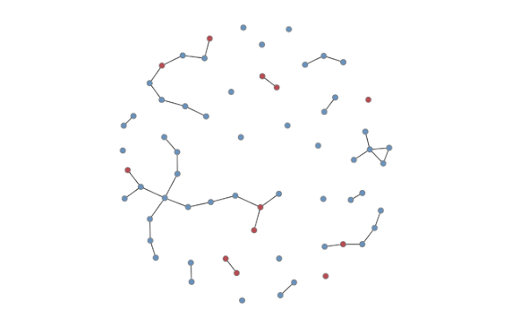
In this random model, there may be concurrency by chance alone, yet without nodal attributes there won't be assortative mixing, or any other relationship-forming phenomenon contingent upon individual attributes. However, in the empiric applications of this we may wish to specify a certain amount of concurrency that is more or less than what is expected due to chance alone. Further, we may also want to favor relationships within groups (homophily). To do this we can extend the basic models by introducing additional network terms in the formation model. See help("ergm-terms"). In all cases, after the network model is estimated and simulated, we need diagnostics to see if the relationship formation patterns met our expectations. This is done by capturing the output from the netdx function, allowing for a variety of goodness of fit tests. In particular, we look to see that the expected value of our network parameters was accurately represented in the (T)ERGM. Once we are satisfied the network is accurately captured, we can return to the initial question of how do we model infectious diseases transmission in a population. To do this, EpiModel includes a netsim function. In addition to specifying the (T)ERGM as an input parameter, we specify information concerning characteristics of disease transmission, which, depending on the type of model (SI, SIR, etc) one is constructed may include per-act probability of organism transmission, duration of infectivity, number initially infected, intervention effectiveness, and so on. Specifically, these are specified in the param.net function (epidemic parameters), init.net function (initially infectivity), and control.net function (aspects of the simulation). After modeling an infectious disease transmission in a social network (above graph), it is then possible to calculate incidence, prevalence, an epidemic curve, R0, and various other metrics used in outbreak investigations.

Cite: Goldstein ND. Social Network Analysis in Epidemiology: Part 3. Sep 1, 2016. DOI: 10.17918/goldsteinepi.
