Testing the Distribution of Disease Cases over Time
Real problem I encountered recently...
Suppose we have X number of cases of disease distributed among Y groups. Seemingly a simple problem, how do we statistically test whether the distributions are independent, or there is some group with greater (or fewer) cases? Let's make this more concrete. Say we're looking at seasonality of flu. Our data is univariate: we have a single variable that indicates the season the case was reported under: Winter (300 cases), Spring (200 cases), Summer (100 cases), Fall (250 cases). We need to setup a statistical test as follows:
H0: Proportion of cases in each season is equivalent
Ha: Proportion of cases in any season differs
Assume independence of groups here (e.g., the number of cases in Fall won't affect the number of cases in Winter, which we know isn't the case, but for didactic purposes we'll assume). The hypothesis test is actually checking:
H0: Proportion of cases in each season is ~25%
Ha: Proportion of cases in any season is not ~25%
The precision around the 25% proportion is defined by the size of the groups in this simplistic analysis. To run this in R code requires an equality of proportions test, with the hypothetical data created as follows:
cases = (N_cases_Winter, N_cases_Spring, N_cases_Summer, N_cases_Fall) = c(300,200,100,250)
And the hypothesis test: prop.test(cases, rep(sum(cases),4)). The code rep(sum(cases),4) simply says there are N total cases possible in each of the four seasons; that is, it's computing the proportion of cases across each season. And that's it: the global test will give you a very basic answer to the question: Are the distribution of cases equal? We can't say much else. Perhaps we can present the data with a bar plot like this:
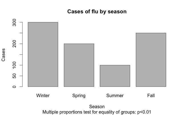
And give a qualitative interpretation along with the statistical test result p<0.01. Let's complicate this a bit and look at the time component for cases of some disease:
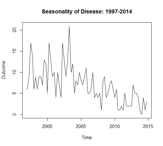
Again, we can give a qualitative interpretation to the plot: the number of cases appears to be declining over the last decade, with some seasonal component (the fluctuations within each year). The more appropriate technique would be a Time Series Analysis. Classic time series analyses decompose the data into an overall trend (controlling for season), a seasonal component, and some remainder (residuals). This can be easily specified into an R "time-series" object via the command: cases_ts = ts(cases, frequency=4, start=year), where the frequency specifies the fluctuations within the year (4 would be seasonal, 12 would be monthly, 52 weekly, and so on). Of course your data need to fit the frequency, as it won't automatically do this for you. The hypothetical plot above is was created with a simple plot.ts(cases_ts) command.
The next step may be to separate the data into its constituent parts, namely the trend, season, and error via the decompose function: decompose(cases_ts, type="multiplicative"). There are two types of decomposition: additive and multiplicative. If the seasonal variation is constant over time use additive decomposition. If the seasonal variation increases (or decreases) over time use multiplicative decomposition, or transform the data (e.g., log transform) to fit the additive assumption. We can plot the decomposed time-series by issuing a plot(decompose(cases_ts, type="multiplicative")) command.
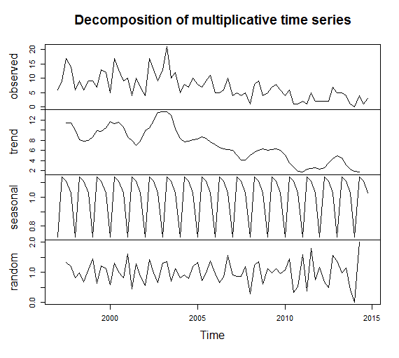
A qualitative inspection shows clear seasonal variation and an overall trend of decreasing number of cases over time. It's also common to explore auto-correlation and partial auto-correlation of time-series data, which essentially says whether there is correlation of the data at different points in time (or are the data completely independent of time, which is the null hypothesis in this analysis).
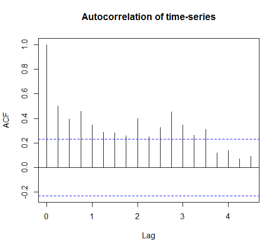
By crossing the dashed lines, there is statistically significant correlation overtime (reject the null hypothesis and conclude there is a trend). At this point there are a wide range of possibilities that are outside of my expertise (please contact me if you'd like to write a follow up post, expanding on time-series analyses!). Smoothing and forecasting is a common next step. This blog post has only scratched the surface of time-series analysis, but has served to introduce the appropriate techniques when testing the distribution of cases over time.
Cite: Goldstein ND. Testing the Distribution of Disease Cases over Time. Sep 11, 2015. DOI: 10.17918/goldsteinepi.