Neal D. Goldstein, PhD, MBI

Bringing census data into an epidemiological analysis

Given the relative ease in running epidemiological models that consider ecological units (see my earlier blog posts on geocoding, multilevel modeling one & two), bringing census data into analysis is nearly prerequisite for identifying public health disparities. In searching for risk and protective factors, it is not enough just to look at individual (person) data; we need to consider systemic and contextual factors as well as potential for interaction between people and their geography. When I have asked students and assistants to pull census data into the analysis, I'm often met with a glazed over look. I think this has to do with the sheer volume of data made available by the U.S. Census Bureau as well as confusion over the geographic units. This blog post is my attempt to demystify the process of linking census data to a preexisting dataset with a specific focus on data from the Census Bureau's American Community Survey.

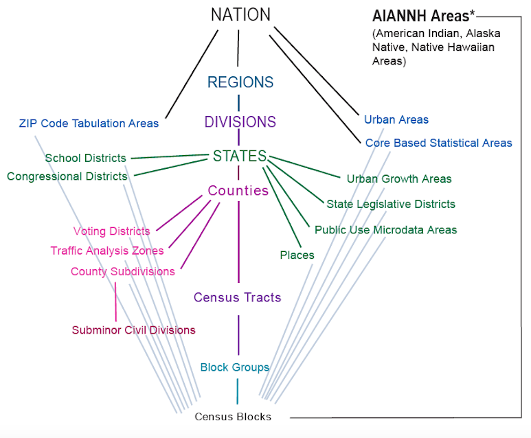
The first thing one needs to understand about the U.S. Census is how the geography is defined. Census estimates are produced for various geographical units, and form a hierarchy (see figure). The smallest census unit is known as a block. This forms the basis for all estimates and other geographic units that arise from census surveys. All areas of the United States can ultimately be broken down into these blocks, and likewise all larger geographic types are aggregates of individual blocks. This is an important concept geographic can be readily transformed from one type to another (we'll return to this in more detail later). Yet one does not always need to start at the block level; census data can be retrieved for a variety of the levels seen in this figure.

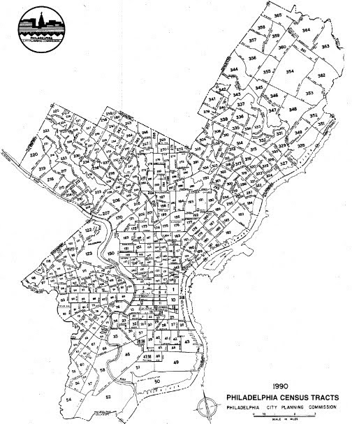
The question of which geographic unit to consider is an important one for both statistical and causal inference in our field. From a statistical standpoint, selecting a unit that is too small will translate to less power to detect statistical differences in areas, especially for nested, multilevel data. Calculating power and deciding on the appropriate ecological unit can be challenging - the University of Bristol Centre for Multilevel Modelling has released software that simulates a multilevel analysis to determine the optimal clustering size with corresponding power estimates. From a causal inference standpoint, one needs to be aware of what census geographies actually represent. For example, census blocks are defined based on "visible features, such as streets, roads, streams, and railroad tracks, and by nonvisible boundaries, such as selected property lines and city, township, school district, and county limits and short line-of-sight extensions of streets and roads." This definition will not necessarily apply to how people live, work, eat, socialize, play, and so on, important factors in public health. Therefore it may be necessary to transform contextual units into ones that are more appropriate for inference. For example, previous work I have done in urban health utilized a mapping between census tracts and neighborhoods in Philadelphia, as neighborhoods more closely aligned to the behaviors I previously enumerated and were public health actionable. Fortunately, there is a defined relationship between geographical entities, and the Census Bureau has created relationship files.

With this understanding of geographical units and the need to retrieve census data, the next question to be tackled is, "Where do I obtain census data?" I have found the easiest place is the Census Bureau's American FactFinder website. There are myriad censuses and surveys conducted by or on behalf of the Bureau. In fact, there are nearly 100 surveys conducted annually and this may be one of the sources of confusion and intimidation in retrieving data that I alluded to at the beginning of this post. Below, I focus on four surveys that are of particular relevance to public health; a comprehensive list of surveys conducted by the Census Bureau can be found here.

• American Community Survey (ACS). This is an annually updated cross-sectional survey at the community level, intended to focus on the changing dynamics within a given area. It is relatively new and community statistics can be obtained for a single year or multi year (3- or 5-year) periods. Single year estimates are available from 2005 on, and 5-year estimates started in 2010. The multi year estimates are designed to average out the per year changes. This survey is my go to for retrieving typical census data including sociodemographic and economic characteristics of an area.
• American Housing Survey. While the ACS includes some information about housing, the American Housing Survey is a much more comprehensive look at wide range of housing subjects. Its longitudinal design allows the research to track trends and changes within the same group of respondents.
• Decennial Census. The only survey official chartered by the U.S. Constitution, this once every ten year census primarily serves for measuring population size and growth for the purposes of redistricting (altering, adding, or removing geopolitical boundaries) based upon population change. The decennial census also includes abundant data on sociodemographic and economic characteristics of an area. It last occurred in 2010, and will occur in 2020, 2030, and so on. One important implication from redistricting is that research studies spanning a decennial census with ecological analysis may induce a bias from the changing geopolitical units. The researcher should consult the census temporal relationship files that align the changing boundaries. There are three possibilities: 1) the census geography is unchanged (the majority of cases), 2) the geography was divided into smaller units (such as due to population growth; the second most common), or 3) the geography was aggregated from smaller units (such as due to population decline; the least common).
• Population Estimates. This survey is particularly useful for obtaining the "denominator" data for various epidemiological measures of health. From the program's website, "Demographic components of population change (births, deaths, and migration) and demographic characteristics (age, sex, race, and Hispanic origin) are produced at the national, state, county, Puerto Rico Commonwealth and municipal levels of geography. Each year, the Population Estimates Program utilizes current data on births, deaths, and migration to calculate population change since the most recent decennial census, and produces a time series of estimates of population." While population denominator data can be found in the ACS (and generally where I pull these data from), it is the Population Estimates program that yields the official estimates.

To access the publically available survey data, I prefer the Advanced Search feature on American FactFinder, and further drill down by the dataset name. Available datasets for a given year can be found under Topics. If your research study were for a single year, I would pull the one-year estimates that align closest to the study dates. If the research study were to span multiple years, the 3- or 5-year ACS estimates may be most appropriate for single measures of Census data, while individual year estimates may provide a more accurate picture of yearly temporal changes. Longer periods of time require further consideration: is it yearly changes that are important or some overall sense of community characteristics? After the dataset is selected, we can then select the geographic type. The most common geographic types default in the drop down selector. You can pull data from as broad as national estimates down to individual census blocks (see hierarchy figure above) and all units in between. Depending on the dataset, some of the geographic units may not be available. Once the geographic type has been selected, you then specify whether the census measures should be pulled for a specific area (such as a State) or for all areas; again, your study population will dictate this selection. At this point, the results will display one, or more likely many, tables that contain the census data (i.e., individual variables). There are a few different ways to go about identifying the tables of greatest relevance (i.e., the ones with the variables you want). The search results can be refined by typing in a topic or table name in the search bar at the top. Many of the tables present results stratified by specific indicators, such as age, sex, and race. The type of data present can be inferred from the Table ID. For the ACS, the first letter indicates the type of table, such as B for the base tables, and S for subject tables. The next two digits identify the subject name, for example 01 indicates data on age and sex. In general it is easiest to start with the broadest tables and if insufficient detail is available, retrieve the more specific tables. The data can now be downloaded and linked to an existing research dataset. While FactFinder provides tools for refining the data on their website, I find it easiest to download the raw tables as stand alone CSV files. The GEO.id variable within each Census table allows them to be readily linked together, and potentially to the external data as well. If your external data has Federal Information Processing Series (FIPS) codes, it is straightforward to merge with the downloaded Census data. Without a geographic identifier such as the FIPS code, one can match on the name of the geographic areas, provided a unique matching identifier can be created (for example, state plus county name). To further understand the geographic identifiers, consult the census website.

One last note concerning the different geopolitical units available: as mentioned earlier, we may occasionally need to transform the geography from one unit to another. Census conveniently provides relationship data, that show 1) how the same type of geography changes over time (comparability), and, 2) how two types of geography are related for the same time period. This note is concerned with the latter type of relationship. Although it is straightforward to aggregate and de-aggregate data over different geographic units, doing so may mask important differences. For example, if you averaged county data to the entire state you may be masking important county-level differences. Likewise if you took county-level data and assumed all census tracts within were equivalent, you may be masking important census tract-level differences. For the researcher who needs to redefine the geographic units, I refer the reader to two sources that may provide useful. When multilevel data are available for population health surveys, Zhang et al. provide a small area estimation methodology, while if only ecological level data are available, Hao et al. provide an elegant solution.

Cite: Goldstein ND. Bringing census data into an epidemiological analysis. Sep 5, 2017. DOI: 10.17918/goldsteinepi.